Measurements made by 3 similar measurement sets in 15 localities in more than 4 years are the main data source. Static pendulum (pendulum with an absorber absorbing pendulum own swings) using 2D static optical contact-less sensor was used for gravity variation measurements.

The basic conclusions are:

A component of gravity interaction different from Newton’s gravity exists on the Earth surface.
Measured quantity includes great irregular component. Irregularity has pink noise (1/f) character.
Measured quantity includes great regular component with 24.00 hour basic period.
Absorption (shielding) effect caused by material between the gravity source and the measurement device was recognized. Gravity shielding effect value of concrete was estimated.
Space dependency of measured quantity is significantly different from Newton’s gravity. Strong altitude dependency and dependency on surrounding material features was recognized.
It was formulated hypothesis that force interaction of gravity field dynamic component can be proportional to time integral of interaction.
The measured features of the gravity interaction component don’t correspond to Einstein’s idea of the dynamic gravity behaviour.

PACS numbers: 91.10.Pp, 04.80.-y

Introduction

Today’s physics have used well-proved Newton’s law to describe gravity effects for more than three centuries. Newton’s law was very well proved in vacuum. It describes very precisely space orbs movement (Kepler’s laws are a special case of Newton’s law). Theoretical tidal forces can be derived from Newton’s gravity law too.

Gravity field on the Earth surface has two parts according to the Newton’s gravity law. The first part is constant static standard gravitational acceleration. It has fixed strength and fixed direction. The second part is dynamic tidal field component with maximum amplitude approximately 10^-7 of the standard gravitational acceleration.

The tidal gravity component is uniquely determined from space orbs positions, primarily from the Moon and the Sun positions against the Earth. Other physical values like Earth geometry, Earth elasticity, ocean and land interaction, water dynamics, coastal shape, resonance etc. are taken into account in more precise computing of tidal effects. The tidal force field is independent on the altitude and the position on the Earth surface if the change of altitude or position is small in comparison to the dimensions of the Earth. Tidal force field is similar in area of million square kilometres.

Resulting from Newton’s law it is nonsense to measure gravity field variations on the Earth surface by the measurement device which has sensitivity comparable with maximum tidal force amplitude. It is nonsense to measure this field on or above the Earth surface where many other “disruptive” effects exist.

But seemingly nonsense measurements are the topic of this article.

Newton’s gravity law describes static gravity interaction behaviour. It means Newton’s law does not deal with gravity field propagation velocity. It does not describe any gravity effect connected with finite gravity field propagation velocity. It supposes de facto unlimited gravity field propagation velocity with no effects connected with the field propagation. A. Einstein tried to fulfil the gap in early 20th century by general relativity theory [1]. The theory is based on light velocity invariance i.e. on Lorenz transformation [2]. A. Einstein formulated an idea: “the geometrical nature of the world is shaped by masses and their velocities”. Gravity waves are expected as the result of Einstein’s theory [3]. A bright experimental proof carrying conviction of Einstein’s gravity theory is still expected.

Earth’s gravity field was and is directly or indirectly measured. Measurement areas, measurement sensitivity and evaluation techniques are different to the ones described in the article.

Modern technology, especially information technology enables accessible way to measure gravity field variations with acceptable resolution and precision for long periods of time and with sufficient number of samples. It enables gravity measurement in different localities including localities generally supposed to be absurd by relative simple and available way.

It enables efficiently evaluate great amount of data, check the credibility of the data and used new tools. It is possible to use automatic measurement, numerical methods like digital filters, parametric transformation [4], FFT [5], STFT [6, 7], and numeric models [8, 9, 10]. Last but not least; Internet enables quick and very productive access to information and data [11, 12].

Many well-known nature effects without credible physical models exist on the Earth surface. Some of them can be influenced by some gravity interaction component different from well-known gravity physical law component. It can be weather, earthquake, volcano eruption, ocean tide anomaly, etc.

The hypothetical gravity interaction must have many times greater effects than Newton’s tide forces and many times smaller effects than standard gravity acceleration on the Earth surface.

Unsatisfactory explained gravity effects exist in the Space. It can be amazing similarity of planet orbit planes in the Sun system, the Saturn’s rings flatness or galaxy flat spiral shape. Those effects can not be explained only by the Newton’s gravity law which is spherically symmetric.

Actually known physical laws do not exclude existence of undocumented gravity interaction.

Known gravity laws have many weaknesses, they have many evident or less evident imperfections. Dynamic factor absence in Newton’s law is well known. Absolute “hardness” of Newton’s gravity field is supposed. Newton’s field must pass through any material without any change. It should radiate through any material like through vacuum. It is historically known as the idea of the Ether (Aether). This feature was not yet experimentally proved or eliminated. Newton’s law was proved only in vacuum and partially in situations with relatively thin air layer [13] or very close to the Earth surface (continental tide measurement). Gravity constant is supposed to be fixed in any material and other correction coefficients or effects are used to bring measurement results and theory agreement [14, 15].

Gravity field interaction dependency on different materials was never disproved. Effects like amplification, attenuation, reflection, refraction or material dependent gravity field spreading velocity was never disproved. The material dependent gravity field spreading velocity can be connected with many interesting gravity effects and “anomalies”.

Gravity measurement is still interesting in modern physics.

Repeated effort to measure and prove theoretically predicted relativistic gravity waves has been unsuccessful until now. The international LIGO project [16] is important representative of those activities.

The gravity waves detection principal used in the project is based on unproved hypothesis of gravity field “absolute hardness”. The experiment assumes that relativistic gravity waves go through every material used for measurement device construction. The device is constructed to enable extremely low movement detection of measurement masses caused by special type of relativistic gravity waves with assumed behaviour. These expected movements must be selected from other many times greater “noise” movements caused by external impacts. The device is constructed to enable mass movement measurement in frequency range around 100Hz.

No expected waves have been detected in the paper creation time in spite of first scientific measurements were planed to start in begin of the year 2002.

The second direction is more precise measurement of the Earth’s gravity field and its time difference. The goal is better understanding of Earth’s gravity field behaviour. Actual international project GRACE [17] is important. It brings interesting data describing Earth’s gravity field abnormalities. The project is based on precise measurement of distance between two satellites orbiting in altitude 100-500km. Gravity acceleration anomalies are recalculated from distance measurement using known physical laws.

Data are sampled in different satellite cycle in different localities. Gravity field in altitude hundreds km is measured repeatedly with period about weeks (in the same locality). No continuous gravity measurement is made directly on the Earth surface in the project.

Many tide measurement are connected with gravity measurement. Continental tides can be measured by tilt measurement, stress measurement or by direct gravity measurement. All these measurements are made as deep as possible. The deepest tide measurement station was about 1300 m under terrain level. It is known that tide measurements are affected by systematic errors with 24.00 hour basic period (S₁ wave). This “error wave” is supposed to be caused by weather impact (meteorological wave). Localities which has S₁ wave lower than 5 times of the maximum theoretical S₁ value (at the latitude around 45-50 degrees) are supposed to be good locality for continental tides measurements. S₁ value greater than 30 times of value in “good stations” (i.e. tilt greater than 0.01”) can be measured in shallow stations (even in depths under 20m) [18].

Newton gravity constant measurement on the Earth surface is not supposed as fully solved question [13], even though the first measurements were made more than 200 years ago.

The text describes experiments designated to prove or disprove existence of undocumented gravity effects on the Earth surface. The experiment results can prove or disprove some generally accepted assumptions or hypothesis used in known theories and physical laws or their interpretations.

Measuring device and measurement method

The gravity field time variations on the surface parallel to the ideal Earth surface i.e. in the plane tangential to reference ellipsoid in the measurement point i.e. in horizontal plane were measured by the displacements measurement of the static pendulum. The static pendulum is a weight fastened to a fixed hanger and calmed in stable state by a liquid absorber absorbing the pendulum’s own swings.

Three similar measurement devices working in 15 different localities were used more than 4 years.

More detail description of measuring device and measurement method together with results processing is described in appendix A – “Measuring Device and Measurement Method”.

Measured results

Basic measured results are described in this section. More comprehensive description of measured results can be found in appendix B – “Measured Results, Reproducibility and Space Dependency”.

Waveform

Measured displacements time sequence shows time dependent quantity.

Irregular component presence and seemingly random periodic displacements with 24 hour period superposition are the basic characteristic features of measured displacements.

Maximal amplitudes of measured periodic component were greater than 3x10^-5 of standard gravity acceleration (i.e. about 300 mms^-2, thus about 30 mGal or 3x10^-5 Radian, thus about 6” – angle seconds). Examples of measured displacements time dependency are displayed in figure 1.

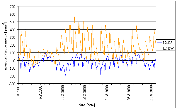
Figure 1 – Time dependence of measured displacements in L2 locality – August 2000. L2-NS is measured displacements component in north-south direction in L2 locality. L2-EW is measured displacements component in east-west direction in L2 locality.

Short-time variance of measured displacements is time dependent. The maximum to minimum variance ratio is greater than 5:1. Comparable variance values can exist for several days or several tens of days. Variance value change can be quick or slow.

The figure 2 shows 3min variance of measured displacements in time interval with quick variance changes.

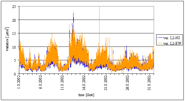
Figure 2 – Time dependence of measured displacements 3min. variance in L2 locality – August 2000.

Spectrum

Spectral analyses of measured displacements give following results:

Significant frequency spectral part has pink noise (1/f) nature.
Spectrum contains 24hour, 12hour, 8hour and 6hour significant spectral lines
Those spectral lines are time dependent with 1 year time period
Spectrum contains 1 year site spectral lines and in some cases small ½ year site spectral lines.

Basic spectral characteristics are shown in figure 3.

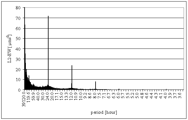
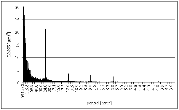
Figure 3 – Total spectrum of measured displacements component L2-EW and L2-NS – May 2000 – October 2004.

Trajectory

Measured displacements periodic component creates trajectories in horizontal plane.

Measured trajectories were frequently similar to slim ellipse. Size and orientation of the measured trajectories were very different.

Trajectories from all measured localities are in the figure 4. Time interval of every trajectory is different. Displayed results were not measured simultaneously.

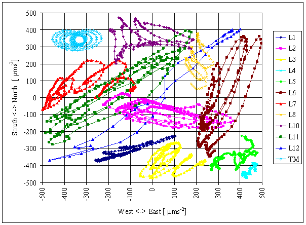
Figure 4 – Measured trajectory in all localities. Periodic movement is superpositioned with irregular movement. Time periods with minimal influence of irregular superposition and maximal periodic movement amplitude were selected from measured results. The measurement in some localities did not enable select ideal time period and time period with great irregular shift had to be selected. This is valid especially for localities with small amplitude of periodic component.
Results from L9 and L13-L15 are very close to L2 results. Those results were not displayed to simplify the figure.
Analogous 100x multiplied trajectory of theoretical Newton’s tide acceleration vector TM is displayed in upper left corner. The trajectory was computed for locality L1-L15. The localities are close each other with respect of Newton’s tide acceleration, that difference in tide acceleration vector trajectories can not be identified in the figure.

Phase

Time position of measured displacements minimum or maximum value in the period (phase) does not differ very much in one locality. These positions are constant in whole measured time period – more than 4 years. No time dependent phase shift was recognised in majority of measured localities.

The phases differ significantly in different localities. In some cases phases differ in different seasons in one locality (see appendix B – “Measured results, Reproducibility and Space Dependency for details).

Measurement results show, that displacements phases are close each other in two separated “phase groups”. It is valid for north-south component and for east-west component as well.

Very interesting results can be analysed from phase and orientation of measured trajectory.

Trajectory orientation is not the same in all localities. Orientation is the same like the virtual Sun orbit in the measurement plane in some localities. It is opposite in different localities.

Phase comparison with respect to the Sun relative position on the sky in localities where measured trajectory orientation is equivalent with the Sun trajectory orientation is interesting.

Measured trajectory in L3 locality follows the Sun movement like pendulum weight was attracted by the Sun i.e. measured displacements tend to the Sun. Measured trajectory in L6 locality follows the Sun in opposition like pendulum weight was repelled by the Sun i.e. measured displacements tend from the Sun.

Measured trajectories with opposite orientation show different position of the same time interval trajectory segment with respect to the trajectory centre.

The conclusion must be deduced from the analyses: Measured displacements are not based on Newton’s gravity interaction between the weight and the Sun.

Space dependency

Measurements were made in 15 different localities. The locality positions vary each other in geographic positions and in altitude above surrounding terrain. Maximal distance between two localities was about 100km. Minimal distance was less than 1m. Locality altitude was from about -3m (3m below terrain level) to about 20m above terrain level. Some localities differ only in altitude. Some localities differs only in horizontal position and are very close each other. All localities were placed about 50° north latitude and 15°east longitude.

Significant similarities between simultaneously measured displacements in different localities were identified. It was not exact match between measured displacements. Significant difference in amplitude and phase was recognised in relatively very close localities (distance several meters).

Conclusion was made: Measured displacements are strongly dependent of on altitude relative to surrounding terrain level.

Time dependency

This section describes analysis results of measured displacements time dependency in different time scales.

Long-term dependences

The first analysis deals with long-time stability of measured displacements trajectory in one locality.

Measured displacements results from L2 locality in selected days were used for the analysis.

The day selection criteria are:

The day is close to astronomically important moment (equinox or solstice)
The day with minimal weather change influence (sunny day without clouds)

Comparison results are in figure 5.

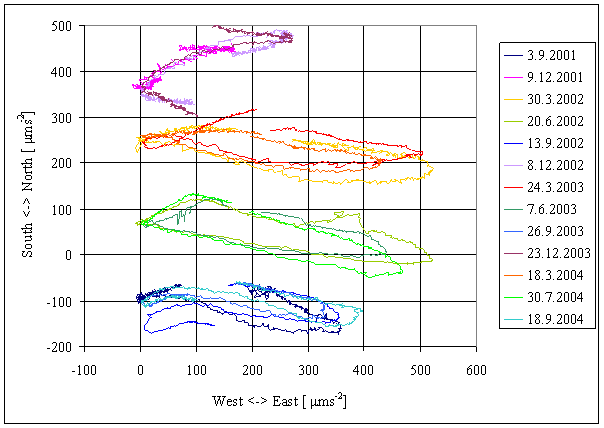
Figure 5 – Measured long-term trajectory dependency in L2 locality. Separate trajectories from different days are shifted by individual offsets. The offsets were selected only for the figure readability and have no physical meaning and no relation with irregular component.

The results show long-term time dependency of measured trajectory. The trajectories change during the time with one year period. This dependency is periodic and reproducible.

The trajectory changes its amplitude, orientation in the plane and shape. The effect was identified in other locality too.

Detail comparison of external effects periodic components with measured displacements showed important relation between L2-EW measured displacements periodic component and some external effects quantities (see appendix C – “External Impacts” for details).

Following part of the paper deals with interesting external quantities relationship in L2 locality i.e. internal temperature T-int (air temperature close to the measuring device weight and sensor), external air temperature T-ext, Sun radiation RA-uexp (both close to the external building surface) and Sun radiation time integral intRA-uexp (numerically integrated from RA-uexp) (see appendix B and C for more detail experiment configuration and external quantities description).

Analysis results are in table 1. 24hour periodic component amplitude of measured displacements and compared quantities were computed as 24hour variance of the signal (always in 00:00 – 24:00 UTC time interval).

	L2-NS	L2-EW	RA-uexp
T-int	0.124	0.260	0.255
T-ext	0.502	0.855	0.846
RA-uexp	0.531	0.878
intRA-uexp	0.495	0.894	0.930

Table 1 – Correlation of selected external effects and measured displacements 24hour amplitude in L2 locality.

Good correspondence between 24hour amplitude of T-ext, RA-uexp and intRA-uexp external effects with L2-EW measured displacements is result of correlation analysis. Only T-int shows low correlation. The greatest correlation is between L2-EW and intRA-uexp.

The correlation is greater than correlation between Sun radiation amplitude (RA-uexp) and external temperature amplitude (T-ext). The table contains correlation between RA-uexp and intRA-uexp (two “images” of the same physical quantity) computed by the same method as other correlations for comparison.

L2-EW correlations are essentially greater than L2-NS correlations. It corresponds with appendix C - “External Impacts” conclusions based on spectral analysis.

Season/ Year	I	II	III	IV
2001			0.930	0.835
2002	0.955	0.916	0.920	0.790
2003	0.936	0.942	0.922	0.762
2004	0.932	0.944	0.929

Table 2 – Correlation of 24hour amplitude L2-EW and intRA-uexp in different seasons in 3 years time interval. The seasons were constructed this way: One year was divided into 4 seasons. Every season was symmetrical to the equinox or solstice. Season I is from 10^th February to 9^th May, season II is from 10^th May to 9^th August, season III is from 10^th August to 9^th November of corresponding year. Season IV is from 10^th November of corresponding year to 9^th February of the next year.

The table shows, that correlations in every season is better than total correlation except all autumn-winter seasons (season IV). It could be explained by the smallest 24 hour periodic component amplitude in the season and relatively greatest influence of irregular component superposition.

Time dependency of 24hour amplitude ratio between L2-EW measured displacements amplitude and Sun radiation integral (intRA-uexp) amplitude is in the figure 6.

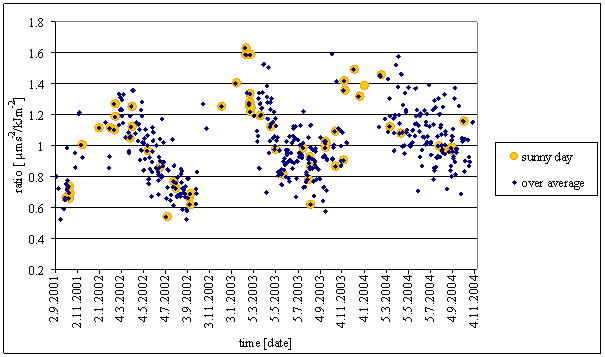
Figure 6 – Time dependence of L2-EW to intRA-uexp 24 hour amplitudes ratios in L2 locality. The graph displays only selected days ratios:

Sunny day – the day with full day sunny weather (without clouds),
Over average – the day with both amplitudes greater than average amplitude.

Selected days must be used to minimise error influence of irregular component. Sunny days were selected to eliminate cloud shielding effect. Over average days were selected to minimize pink noise and measurement errors in small amplitudes ratio.

The results can be formulated:

Amplitude ratio is not constant
Amplitude ratio time dependency is periodical function
Maximum to minimum values ratio of the function is greater than 2:1
Time period is one year
Maximum value is close to spring equinox, minimum value is close to autumn equinox

Short-term dependences

L2-NS and L2-EW measured displacements component time relation with external temperature T-ext and Sun radiation RA-uexp in selected days were analyzed.

The days with rapid and strong weather change were selected from measured results.

Measured displacements with external effects time dependency from those days are displayed in figure 7. 3 minute averages are used in the figure.

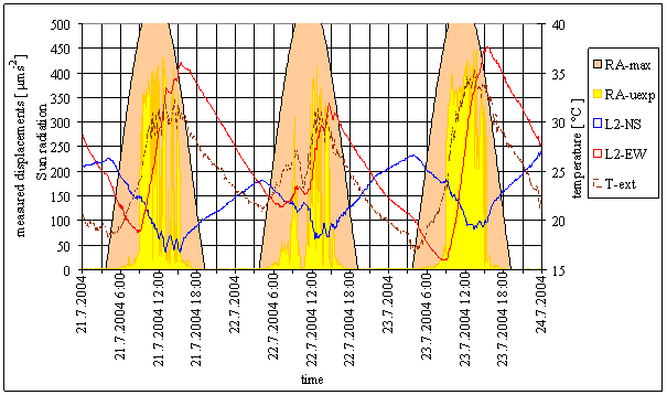
Figure 7 – Short-term dependency between measured displacements, external temperature and Sun radiation in L2 locality – day 21.7.2004 - 23.7.2004. Sun radiation graph scale respects measured displacements scale by constant coefficient to enable relative comparison. Measured displacements offsets were adjusted for readability of the figure.

The graph shows clearly time relation between Sun radiation and measured displacements. Both L2-EW and L2-NS measured displacements components changes theirs shapes in the weather change moment. It can be seen, that measured displacements shape differs in full Sun radiation time from the shape in low Sun radiation time (moderated by cloudiness).

It can be seen, that delay between external temperature T-ext events and measured displacements L2-NS and L2-EW events is not constant. The time connectivity with Sun radiation exists in all cases.

The results implicate hypothesis: Local Sun radiation and measured displacements are affected by the common cause.

Cloudiness can be the common cause. The clouds between measurement locality and the Sun can cause Sun light radiation modification simultaneously with measured quantity modification in L2 locality.

Sun radiation integral

Waveform time consistency and correlations results show greatest consistency between L2-EW and intRA-uexp computed from reconstructed Sun radiation RA-uexp by the equation (1):

(1)

where is time constant relevant to frequency characteristic breakage frequency, is angle speed .

Digitally filtered waveform intRA-uexp computed from measured Sun radiation RA-uexp in L2 locality using equation (1) compared with simultaneously measured displacements L2-EW in several time intervals shows good correspondence of irregular waveforms.

The comparison verifies hypothesis, that measured displacements L2-EW are similar to Sun radiation time integral intRA-uexp and vice versa.

The implications from the section are:

Measured displacements L2-EW are very similar to the Sun radiation time integral in measurement locality (with respect of local building shielding effect).
24hour amplitude L2-EW to intRA-uexp ratio changes its value more than 1:2 during the year.

Maximum value is close to spring equinox, minimum value is close to autumn equinox
Amplitude ratio time dependency is periodical function with one year time period
Measured displacements L2-EW and L2-NS reacts in very short time (in a few minutes) to weather change.

Notes to implications:

Cloudiness is probably common cause of measured displacement waveform change and Sun radiation change.
Shielding effect of building and clouds can explain measured effects.
Measurement device was placed in the room with minimally 25 cm wide ferroconcrete walls without any window. It means that measured quantity event must pass through the concrete walls in time shorter than a few minutes.

Other measured features and results from different localities including near locality verification experiments are described in appendix B – “Measured Results, Reproducibility and Space Dependency”.

External impacts

Possible local dependency of measured displacements on other physical impacts in measurement locality are analysed in detail in appendix C – “External Impacts”.

The analysed quantities were: temperature (internal, external and independently measured), Sun radiation (locally measured, independently measured, ideal and shielding effect modelled), atmospheric pressure, dew point temperature, wind speed, air relative humidity and combinations. All the effects were analysed by black box analysis using linear dynamic system, nonlinear static and nonlinear dynamic systems working hypothesis.

Specific analysis of anthropogenic impacts, subsoil tilt, building deformation impact and wind speed were made.

Basic conclusions from appendix C are:

Dominant cause of measured displacements is different from all analyzed external effects. Every analyzed external quantity has no dominant impact to measured displacements.
The unknown cause has dominant impact to the measured displacements; measured quantity has its own laws. The laws are different from local dependency on any analyzed external quantity or their combinations.
Any external quantity impact to measured displacements was not fully eliminated. This impact can cause measurement errors.
Those measurement errors have not sufficient value to prevent studying the unknown quantity qualitative features.

Following features of unknown quantity were recognized:

The best correspondence of L2-EW spectrum is with local radiation RA-uexp and modelled local radiation SSS (including building shielding) spectrums (with respect of integrating transfer function).
All other signal spectrums give worse correspondence.
L2-NS component spectrum is different from any other analysed spectrums.
Measured displacements have different noise type than Sun radiation (integrating transfer function must be used)
Only L2-NS component enables considering time independent transfer function f of separate irregular signal component temperature dependence.
The L2-EW measured displacements component does not enable any transfer function approximation of irregular signal component by any type of time invariant transfer function f.

Conclusions

Identified measured results summary

Identified measured displacements features can be summarised:

Time dependent physical quantity which interacts with pendulum weight was repeatedly measured in all different localities and by different measurement devices.
The physical quantity was measured in the horizontal plane i.e. in the plane tangential to the reference ellipsoid in the measurement point.
The measured physical quantity is external time dependent vector. Measured physical quantity interaction with the weight mass is equivalent to gravity gradient direction change.
Two basic components of measured quantity was recognized:

Irregular, random or pseudorandom component with continuous spectrum inversely proportional to frequency (1/f) which can be supposed as a pink noise.
Periodic component with basic period 24.00 hour and seemingly random amplitude.

Following features of periodic component was identified:

Amplitude:

Displacements amplitude can be greater than 3x10^-5 of standard gravity acceleration, thus 3x10^-4 ms^-2 i.e. angle aberration can be greater than 3x10^-5 radian, thus 6” (angle second). It is more than 100times greater value than maximal Newton’s tide generation force amplitude. It is more than 5% of Newton’s gravity acceleration of the Sun on the Earth.
Amplitude is not constant. Amplitude is time dependent. Amplitude time dependency includes irregular time dependency and periodic amplitude dependency with annual time period.

Spectrum:

Spectrum of measured displacements contains basic period of 24.00 hour (15 deg per hour) and important spectral lines with period of 12.00 hour (30 deg per hour), 8.00 hour (45 deg per hour) and 6.00 hour (60 deg per hour). No spectral lines greater than noise with period matching the Moon movement was identified.
All periodic components spectral lines are time dependent. Time dependency period is one year.
Spectrums of orthogonal components can be different. They differ in spectral lines existence and in spectral lines time dependency.

Phase:

Periodic component phase has specific behaviour. Phase can change significantly with respect of locality or time. Phase is very stable in long time period. Very different phases in different localities and different components were measured. Maximums and minimums of measured displacements time positions enable grouping into “phase groups”. Time interval with no maximum or minimum was identified in all measured results.
Opposite phases can be identified in relatively close localities (a few meters altitude difference).
Phase change during year was identified only in one locality and only in one direction component. The phase changes were measured twice a year. The phase change is based on amplitude change of two synchronous signal components with shifted phases. No phase jump or phase movement was identified.

Trajectory:

Periodic component trajectories in horizontal plane match pendulum weight attraction by the Sun in some localities and pendulum weight repulsion by the Sun in other localities. Trajectories with opposite movement orientation than the Sun relative movement were measured in some other localities.
Trajectories are similar to more or less deformed ellipse in many localities. Trajectory circumferential velocity is time dependent in several localities. Waveforms don’t need to be symmetrical.

Time dependency:

Periodic component pseudorandom nature is similar in different localities (similar small and great amplitude sequences). The similarities between more than several tens of km distant localities were identified; even so measurement displacements can be different in many other attributes (e.g. phase difference, different irregular component value or shape, only one axis similarity).
Annual reproducible periodic change of measured displacements in L2 locality was recognised (trajectory orientation, size and shape change). Season dependent change was repeatable recognised in all localities where relevant measurement was made.

Space dependency:

Significant dependency on locality and especially strong dependency on altitude above terrain were identified. Altitude difference of few meters (5 -15 m) caused significant difference in measured displacements. Altitude difference 1m can give recognisable difference in measured displacements.
Significant building influence to measured displacements similar to shielding was identified.

Some regularity was recognised in irregular component. Following features of irregular component was identified:

Short-term time events:

Measured displacements waveform have significant events in relatively very close time (in less than several minutes) to change of Sun radiation in the measurement locality. The events repeatedly exist even though the measuring device is separated from the Sun by minimally 25 cm thick ferroconcrete walls.
The events exist in times of start or end of Sun radiation shielding (caused by the building) in sunny days. The events are missing in cloudy days.
The events exist in times of rapid Sun radiation change caused by clouds in days with changing weather. Every rapid Sun radiation change in irregular time has synchronous measured displacements event.
The reaction is not directly connected with the Sun radiation direction. It coheres with total Sun radiation amplitude.

Long-term irregularity:

No reliable long term dependency of the measured displacements irregular component was found. Annual period can be unreliable identified in L2-NS component. The measurement results can be significantly corrupted by accumulated offset errors in that long-term measurement.

Correlation:

The greatest correlation exists between measured displacements L2-EW and Sun radiation integral in L2 Locality. The correlation value is higher than 0.9 in ¾ of annual period. Correlation value is about 0.8 in winter solstice season.
Measured displacements amplitude to Sun radiation integral amplitude ratio changes its value with annual period in range about 1:2.
Equivalent significant correlation does not exist in measured orthogonal component in the same locality.

Relation to other irregular quantity:

All other compared external quantities have no reliable relations with measured displacements.

Reproducibility:

No similar irregular displacements can be reliable measured by one measuring device in different time.
Irregular component is included in measured physical quantity and has vector character in all localities.
All simultaneously running measuring devices in near localities give similar results of short-term and medium-term irregular component independently on the measuring device orientation. No long-term experiment was made to test long-term irregular component reproducibility.

Physical conclusions

Experiments results and linked analysis give following physical conclusions:

The reproducibly measurable physical quantity exists.
The quantity is irregular in time.
The quantity is not caused by any analysed quantities or their combinations.
The mass impacts of measured quantity and gravity field compliance were verified:

Direct proportion between acting force value and test weight mass (experimentally verified with mass range greater than 1:2)
Direct proportion between measured distance difference in horizontal plane and hanging wire length (experimentally verified with length range about 1:2).

Measured quantity partially depends on common cause with Sun light radiation. Sun radiation integral gives very good agreement with one measured quantity vector component. Second quantity vector component has different behaviour.
Measured quantity is not caused by known feature of electromagnetic field.

Other well known important facts:

Electromagnetic field is described by experimentally well proved physical laws including static and dynamic behaviour and including material features.
Gravity field is described only by static physical law well proved only in vacuum. Gravity field dynamic and material dependence was not successfully experimentally proved yet.

The measured quantity can be explained as time dependent gravity field on the Earth surface. The measured features are essentially different from theoretical Newton’s tide forces i.e. the quantity is different from Newton’s gravity interaction. The measured displacements are not in conflict with Newton gravity filed if superposition with other gravity field component is considered.

All above findings are not in conflict with known independent measurement results implemented in other localities sometime in the past.

The basic recognised physical features of the quantity are:

Time dependent vector in horizontal plane,
Superposition of irregular pink noise component and periodical 24hour period component with amplitude annual regular change and amplitude modified by pseudorandom multiplicative value,
Strong space dependency in range several meters, particularly altitude dependency above terrain level,
Periodic component amplitude greater than 3x10^-4 ms^-2,
Some effects that can be explain as shielding effect. Estimated building material (concrete) shielding penetration depth (measured displacements interaction is ½ of original value) is about 0.3-0.8m,
Great correspondence of measured Sun radiation time integral with one vector component of measured quantity.

Following essential physical conclusions can be formulated from previous results:

Existence of gravity interaction component different from Newton’s gravity interaction – gravity interaction component with different nature than known Newton’s gravity interaction exists. The component has greater impact on the Earth surface and above the Earth surface than theoretical Newton’s tide forces and lower impact than static Newton’s gravity forces.
Identified gravity interaction shielding effect - identified dynamic gravity interaction component is dependent on interacting body substance. The interaction result depends on presence, material type and shape of bodies in interaction area. The gravity interaction is modified by the materials it passes through. Basic material dependent behaviour value was quantitative estimated for building material (concrete) shielding penetration depth. Cloud shielding effect was identified.
Gravity field includes noise – noise is natural part of body gravity interaction. Existence of noise is not surprising feature of many other physical quantities. It is unusual to think about noise in gravity filed. No known experimentally proved reason exists excluding gravity field noise as integral part of gravity.
Gravity field nature hypothesis – the following hypothesis is formulated. A gravity field component dependent on geometry, masses and material features of interacting bodies exists. The gravity noise is natural feature of body gravity interaction.

Gravity field doesn’t depend only on masses and distance of interacting bodies, but on other body geometry and material as well. Effects like attenuation, amplification, reflection, refraction or other effects on the material boundary or close to material boundary can exist.

Time integral hypothesis - the following hypothesis is formulated. Gravity field component with force effect dependent on time integral of acting gravity field exists. The force interaction can be described:

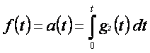(2)

where:

f(t) – unit force time dependency

a(t) – acceleration time dependency

g₂(t) – gravity field component time dependency

It is not known, if the integrating effect is caused by materials between interacting bodies or if it is a feature of the own gravity field interaction.

It was recognized shielding effect of the material. The shielding effect can be described as multiplicative coefficient of gravity field component. The coefficient can be time dependent. Time dependency can be caused by relative movement of shielding mass. Recognized pink noise can be in agreement with time integral hypothesis.

Einstein’s idea of gravity field dynamic behaviour deconstruction – gravity field material dependence recognized from identified shielding effect deconstructs Einstein’s idea: “The geometrical nature of the world is shaped by masses and their velocities. The gravitational equations of the general relativity theory try to disclose the geometrical properties of our world.” [1]. Gravity field material features dependency (shielding) and gravity noise do not correspond with Einstein’s general relativity theory.

Open questions

The paper does not answer some existing questions of gravity. Known question of gravity field propagation velocity was not answered.

New question are opened:

Material dependence of dynamic gravity interaction. Different materials should be tested.
Material dependence of Newton’s gravity interaction. Newton gravity law could be modified by material dependent multiplicative coefficient with unknown value. Some material dependent shielding effect of Newton’s gravity interaction can exist.
Possibility of other gravity effects like gravity refraction or reflections. Other fields give special effects on different material boundary. Similar or different effects should be discovered.
Space dependency of dynamic gravity interaction on Earth surface (local and global)
Earth gravity noise analysis
Described results reproducibility by fully independent measurement

Many interesting implications can be formulated on the described results basis. They can open many other questions.

The Earth is source of gravity noise. The noise has pink noise character of force interaction. The pink noise was independently measured in many physical quantities on the Earth surface (i.e. tide value in many tide measurement stations or weather parameters in great amount of weather gauge stations). Explaining tide pink noise existence by Earth gravity pink noise is unusual but possible. Explaining of weather irregularity by Earth gravity noise is unusual but possible (measured acceleration value acting one hour to a mass generates horizontal velocity about 1ms^-1). Explaining earthquake starting mechanisms or irregular volcano starting mechanism by Earth gravity noise combined with gravity interaction material and space dependency is unusual but possible.

The Earth is source of gravity noise. It can be very surprising idea. Many other many times smaller sources of noise are well known. Why the Earth can not be source of measurable gravity noise? Why the gravity noise can not have the pink noise character of force interaction? Why the noise can not have amplitude comparable with measured results?

Dynamic gravity interaction is attenuated by a mass very quickly. Is the attenuation dependent on the mass material or on the mass density? What is atmosphere gravity attenuation value? What is dynamic gravity interaction value in vacuum?

Can be designed some gravity refractors, gravity attenuators or other gravity modification devices?

Many other experiments and scientific work must be done to answer the questions.

Acknowledgements

I want to thank my wife, my family, and my friends for many-year tolerance, help and support of the research.

References

[1] A Einstein, The Evolution of Physics, Simon and Schuster, New York, 1942

[2] R P Feynman, R.B.Leighton, M.Sands, The Feynman lectures on physics, Addison-Wesley Publishing Company, 1966

[3] J Weber, Detection and Generating of Gravitational Waves, Physical review, Vol. 117, No 1, January 1, (1960)

[4] Feature space transformation for line detection, The Marble Project, Interactive Vision, April 1996,

http://www.dai.ed.ac.uk/CVonline/LOCAL_COPIES/MARBLE/medium/contours/feature.htm

[6] Alan Wesley Peevers, A Real Time 3D Signal Analysis/Synthesis Tool Based on the Short Time Fourier Transform, Department of Electrical Engineering,

University of California, Berkeley, http://cnmat.cnmat.berkeley.edu/~alan/MS-html/MSv2_ToC.html

[7] Signal Processing Toolbox, tukeywin, http://www.mathworks.fr/access/helpdesk/help/toolbox/signal/tukewin.shtml

[8] WG on Theoretical Tidal Model (SSG of the Earth Tide Commission, Section V of IAG, geodynamics), July 1997, http://www.astro.oma.be/D1/EARTH_TIDES/wgtide.html

[9] Markku Heikkinen, On the Tide-Generating Forces, Publications of Finnish Geodetic Institute, No 85

[10] H.G.Wenzel, Earth Tide Data Processing Package Eterna, Version 3.30, Black Forest Observatory, Karsruhe University, 1996

[11] Synoptical meteorology data from the station 11520 Praha-Libuš range 1.4.2000 – 31.3.2003, Czech Hydrometeorological Institute, http://www.chmi.cz/indexe.html

[12] Measured ocean tidal data from different tidal stations, NOAA Center for Operational Oceanographic Products and Services, http://www.co-ops.nos.noaa.gov/co-ops.html

[13] D.Sarkadi, L.Bodonyi, A Gravity Experiment Between Commensurable Masses, Journal of Theoretics, Vol. 3-6, 2001

[14] Christopher Garret, Tidal Resonance in the Bay of Fundy and Gulf of Maine, Nature, vol. 238, August 25, 1972

[15] M.C.Hendersott, The Effects of Solid Earth Deformation on Global Ocean Tides, Geophys. J., E.astr. Soc. (1972) 29, pp 389-402.

[16] LIGO – Laser Interferometer Gravitational Wave Observatory, California Institute of Technology, Massachusetts Institute of Technology, http://www.ligo.caltech.edu/

[17] GRACE – Gravity Recovery and Climate Experiment, National Aeronautics and

Space Administration Goddard Space Flight Center, http://www.csr.utexas.edu/grace/

[18] Paul Melchior, The Tides of the Planet Earth. Second edition. Pergamon Press. Oxford, New York, Toronto, Sydney, Paris, Frankfurt, 1983

[19] Amara Graps, An Introduction to Wavelets, IEEE, 1995, http://www.amara.com

[20] Keith Clayton, Basic Concepts in Nonlinear Dynamics and Chaos, A Workshop presented at the Society for Chaos Theory in Psychology & Life Sciences meeting, July 31, 1997, http://www.societyforchaostheory.org/tutorials.html